Show EOL distros:
Package Summary
This package contains a system to recognize scenes called the Probabilistic Scene Model (PSM). It uses objects and relative poses (relations) between the objects. The realations can be dynamic and each object can be a reference object. The system consists of a training subsystem that trains new scenes and a scene inference subsystem that calculates scene probabilities of previously trained scenes.
- Maintainer: Meißner Pascal <asr-ros AT lists.kit DOT edue>
- Author: Braun Kai, Gehrung Joachim, Heizmann Heinrich, Meißner Pascal
- License: BSD
- Source: git https://github.com/asr-ros/asr_psm.git (branch: master)

Contents
Description
The Probabilistic Scene Model PSM is a system to recognize scenes. It uses objects and relative poses (relations) between the objects. The relations can be dynamic and each object can be a reference object.
The system consists of a training subsystem that trains new scenes and a scene inference subsystem that calculates scene probabilities of previously trained scenes.
Functionality
The Learner collects objects from a database and learns a gaussian mixture model (GMM) with expectation maximization. The GMM represents the relation between to objects. The training process is done offline.
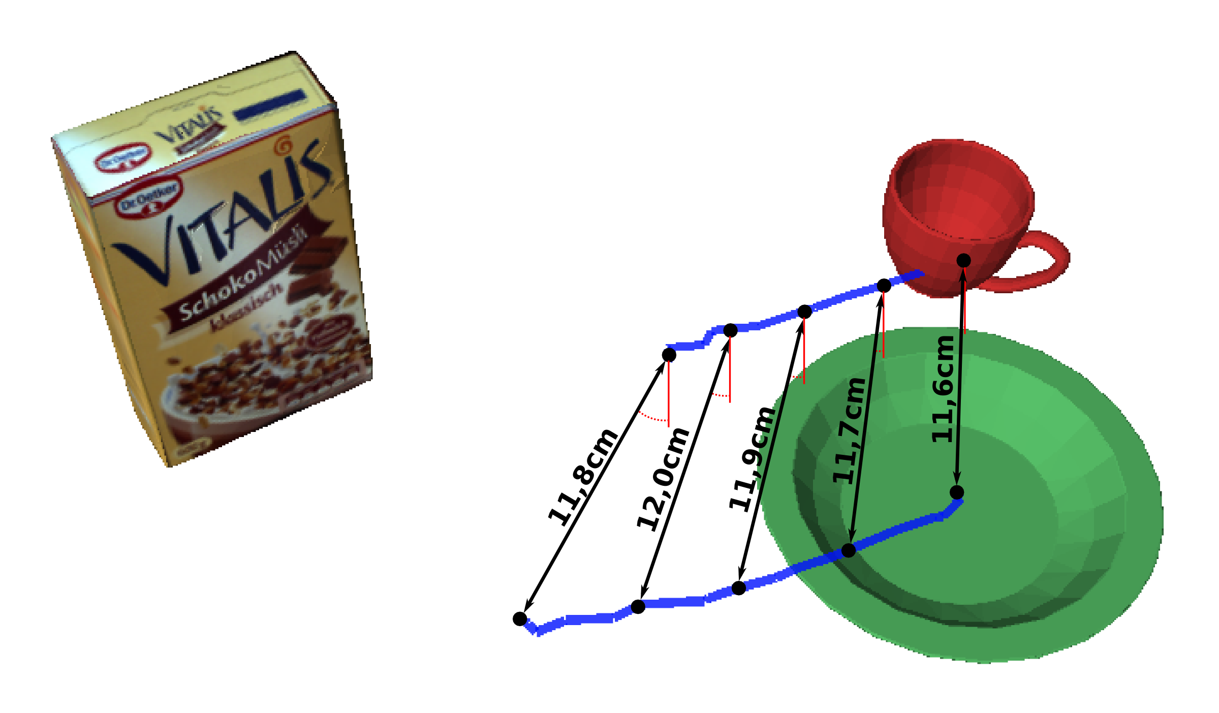
Figure 1: The learner uses observed object trajectories as the basis for its calculations. Here, the blue lines indicate the movement of the cup and plate respectively. Alternatively, combinatorial optimization can be used to find a set of relations; see below.
The learner also learns probabability tables representing the probabilites that an object was not observed in some of the steps of the trajectory used for learning ("Object Existence") or that an object was misclassified as another by the independent object recognizer ("Object Appearence"). The current implementation assumes that every object was visible and correctly classified in every step.
Output: XML File that contains the learned Object Constallation Models (a modified variant of the Constellation Model https://en.wikipedia.org/wiki/Constellation_model), Object Appearence and Object Existence for the new scene.
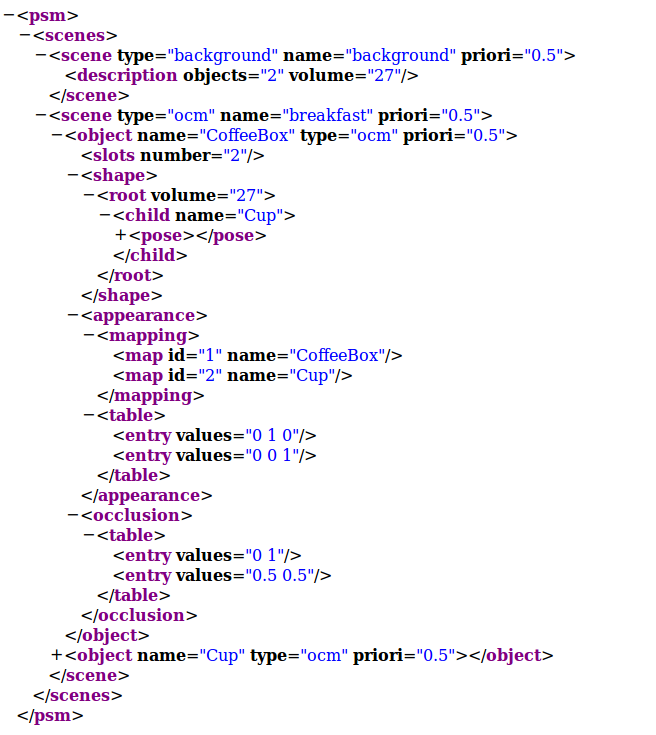
Figure 2: An example for the models created by the learner. The xml-file contains the scene model of a breakfast scene with a coffee box and a cup. The model consists of a fore- and a background scene. The foreground is made up of the two objects containing the parameters for the three terms of the OCM.
The Inference calculates the a posteriori probability of all scenes in the learned scene description xml-file and the background scene given a list of object_msgs. The probabilities are floats that sum up to 1. The inference can be done online.
It uses the GMMs (representing a Bayesian Network) and the probabilty tables.
Since the PSM is a parametric model and the learned models are stored in a human readable xml file, the paramteres of the model can be edited in a text editor and one doesn't need to train a whole new model if e.g. an object should be exchanged with a new one.
Compare asr_psm_visualizations and the general asr_psm tutorial for how the results are visualized.
Usage
Needed packages
asr_relation_graph_generator to select as little relations as possible to fully describe the global neighbourhood of objects during training.
asr_psm_visualizations to visualize the results with RViz and gnuplot.
Needed software
Camera software, object recognition system (e.g. asr_aruco_marker_recognition), asr_kinematic_chain_dome.
for visualization (used by asr_psm_visualizations): RViz, gnuplot
- Eigen
- Boost
- OpenCV2
asr_ism recorder to record object messages into databases
Needed hardware
- Camera (unless the system is called with prerecorded samples which could either be in rosbag or database files)
Start system
Learner: Start ptu_driver, recognition manager, the object detectors and recorders. Then edit the parameters in the learner.launch and finally launch it.
Inference: For online evaluation of the PSM start inference.launch.
You can also run the inference system through the !ProbabilisticSceneRecognition::SceneInferenceEngine. It uses asr_msgs::AsrObject messages and calculates the scene probabilities of the scene that is given via a ros param. Take a look at asr_recognition_prediction_psm/psm_node_server.cpp for an example.
Simulation
The starting process is the same for simulation and real. For simulation, use rosbag play or asr_ism fake_data_publisher to simulate prerecorded or artificially created files.
Real
Use the camera and object recognizers to create object messages.
ROS Nodes
Subscribed Topics
Inference:
/stereo/objects (asr_msgs::AsrObject) for evidences
Parameters
learner.launch:
input_db_file: The database files containing scene samples that should be used for learning.
scene_model_name: Name of the output .xml file containing the model.
scene_model_type: The type of the scene that should be learned. "ocm" be default, since no other types are currently implemented.
scene_model_directory: path to the directory where the resulting model xml file should be stored.
workspace_volume: The volume of the workspace we're working in in cubic meters. Dependent on your recording setup and scene. Default: "8.0".
static_break_ratio: for the relation graph generator's heuristic selecting relations: static breaks are misalignments in angle between two objects at different trajectory steps. If there are more static breaks than static_break_ratio (multiplied with the sample range), two trajectories are considered not parallel. Default: "1.01".
together_ratio: for relation graph generator, which uses agglomerative clustering to build a tree of the relations: if two objects do not appear together in more than together_ratio of the trajectory steps, they are considered not parallel. Default: "0.9".
intermediate_results: whether or not to show intermediate results. Default: "false".
timestamps: whether or not to add timestamps to the result file name. Default: "false".
- _kernels_min_*: the minimal number of kernels per GMM. Default: "1".
- _kernels_max_*: the maximal number of kernels per GMM. Default: "1". A higher number of kernels leads to more precise results, but longer training time.
- _runs_per_kernel_*: The number of separate runs per kernel to possibly improve the resulting kernel. Default: "1".
- _synthetic_samples_*: the number of additional samples to create around every recorded sample. Default: "0".
- _interval_position_*: asr_psm uses sample relaxation to improve results. This parameter determines the interval for the sample relaxation for the position (in meters). Default: "0.50"
- _interval_orientation_*: determines the interval for the sample relaxation for orientation (in degrees). Default: "10".
orientation_plot_path: if this parameter is not set to "UNDEFINED", a gnuplot file for each Gaussian Kernel for orientation in roll, pitch and yaw is written and the gnuplot shown on screen. Since this leads to a lot of plots and files for large numbers of kernels, it is deactivated by default. Default: "UNDEFINED".
max_angle_deviation: for relation graph generator heuristic: the value in degrees above which an angle is considered a misalignment. Default: "45".
base_frame_id: The name of the frame the objects should be transformed to. default: "/PTU".
scale_factor: to enlarge the visualization. Default: "1.0".
sigma_multiplier: multiplier to the sigma of the standard deviation. Default: "3.0".
- _attempts_per_run_*: How often the learner attempts to learn a valid model in each run until it gives up and throws an error. After half the attempts, the learner switches from a generic to a less precise but more stable diagonal matrix as base for the covariance matrices. Use "2" if each matrix type should be tried exactly once and "1" if only a generic matrix should be used once. Default: "10".
*The parameters kernels_min, kernels_max, runs_per_kernel, synthetic_samples, interval_position, interval_orientation and attempts_per_run can be specified for each scene separately by setting "<scene name>/<parameter name>". If unspecified, the default (without added "<scene name>/") is used. This can be done for each parameter separately.
inference.launch:
plot: set true to show the gnuplot bar diagram of the scene probabilities. Default: "true".
object_topic: the topic to get the AsrObject messages from. Default: "/stereo/objects".
scene_graph_topic: the topic to get the AsrSceneGraph messages from. Default: "/scene_graphs".
scene_model_filename: path to the file containing the PSM .xml file.
bag_filenames_list: path to the bag file that contains the learning data.
base_frame_id: The name of the frame the objects should be transformed to. Default: "/PTU".
scale_factor: to enlarge the visualization. Default: "1.0".
sigma_multiplier: multiplier to the sigma of the standard deviation. Default: "2.0" (different from above).
targeting_help: set true to overwrite the visualizations of results and plot the target distributions instead. Default: "false".
evidence_timeout: the timeout for object evidence in milliseconds. Default: "100".
inference_algorithm: the name of the inference algorithm. There are 'powerset', 'summarized', 'multiplied' and 'maximum', which determine how different subresults are combined with each other. Default: "maximum"
runtime_log_path: the path to the directory that should hold the log files containing the runtime outputs for the different scenes. To deactivate logging, remove this parameter from the launch file. Runtime output will then be printed to console. Removed by default.
combinatorial_learner.launch:
A set of relations between the observed objects can be selected via a heuristic based on how parallel trajectories are to one another, as illustrated above. Alternatively, combinatorial optimization can be used to find the relations. During optimization, different relation sets are considered, selected based on the particular optimization algorithm. They are assigned a cost in terms of their average recognition runtime and number of recognition errors, which are calculated by running recognition on a model learned on the relation set against a number of test sets, randomly created observations of the scene objects. In the end, a relation set with optimal cost is returned. This method takes much longer to learn than the heuristical method, but can result in better relation sets in terms of recognition errors.
To use combinatorial optimization, set the optional parameter relation_tree_trainer_type to combinatorial_optimization, like in combinatorial_learner.launch (if the parameter is not provided, the default value of tree is used, which refers to the heuristic. Alternatively, it can be set to fully_meshed. In that case, all possible relations are used, which results in a higher recognition runtime but the best possible recognition accuracy). In addition to several familiar parameters (compare above), a couple of new ones have to be provided, as in combinatorial_optimization.yaml:
optimization_algorithm: type of optimization algorithm to use. From " HillClimbing", "RecordHunt", " SimulatedAnnealing". Record Hunt stores the record and allows to consider worse relation sets if their cost is inside a certain delta. Default: HillClimbing.
starting_topologies_type: type of starting topology (relation set) to use. From "BestStarOrFullyMeshed" (uses the best set of star-shaped relations or containing all relations), "Random". Default: BestStarOrFullyMeshed.
number_of_starting_topologies: number of topologies to start separate optimization runs from. Default: 1.
neighbourhood_function: type of the neighbourhood function to use. The neighbourhood function returns possible sets close to the current one to be considered for the next one to be tested. Default: TopologyManager, no other types available.
remove_relations: whether to use removal of relations as operation in neighbour generation. Default: true.
swap_relations: whether to use swapping of relations as operation in neighbour generation. Default: true. The third operation, which cannot be deactivated, is adding relations.
maximum_neighbour_count: maximum number of neighbours to select in each step. Default: 100.
cost_function: type of the cost function to use. Here, a weighted sum of normalized average recognition runtime an recognition errors (in the shape of false positives and negatives) is used. Default: WeightedSum, no other types available.
false_positives_weight: the weight to give the number of false positives in the weighted sum. Default: 5.
avg_recognition_time_weight: the weight to give the average recognition runtime in the weighted sum. Default: 1.
false_negatives_weight: the weight to give the number of false negatives in the weighted sum.Default: 5.
test_set_generator_type: type of test set generation to use. From "absolute" (picks random observations off the trajectories for each object, for visualization), "relative" (same, but transforms the poses into the frame of a randomly chosen reference object), "reference" (same, but does not transform the reference pose itself. Generates mostly invalid sets, since the reference tends to be far away from the others). Default: relative. See Figure 3 for an example of two test sets.
test_set_count: number of test sets to use to test relation sets against. Default: 1000.
object_missing_in_test_set_probability: probability with which an object does not appear in a test set. Set to 0 to have all objects appear in each test set. Default: 1.
recognition_threshold: threshold above which a relation is considered fulfilled. Scene threshold, above which scenes are recognized as valid: recognition_threshold^(|objects|-1). Default: 1.0e-04.
valid_test_set_db_filename: database file to load the valid test sets from. New test sets are created if this is set to . Default: .
invalid_test_set_db_filename: database file to load the invalid test sets from. New test sets are created if this is set to . Default: .
loaded_test_set_count: how many test sets loaded from the database to use at first. Reduced to test_set_count later, but since some loaded sets may be misclassified and removed, it can be useful to load more than test_set_count (loaded_test_set_count should be bigger than or equal to test_set_count for this reason). Default: 1000.
write_valid_test_sets_filename: database file to write newly created valid test sets to. Test sets are not written if they were loaded from files above or this parameter is set to . Default: .
write_invalid_test_sets_filename: database file to write newly created invalid testsets to. Test sets are not written if they were loaded from files above or this parameter is set to . Default: .
conditional_probability_algorithm: algorithm used to determine probabilities depending on multiple parents. From "minimum" (uses the minimum of the single parent probabilities), "multiplied" (multiplies them, which makes the invalid assumption that they are independent from each other), "root_of_multiplied" (multiplies them and takes the |parents|-th root to keep a consistent range of values), "average" (uses the average of the single parent probabilities). For trees, as from the heuristical method, this is irrelevant. Default: minimum. Compare Figure 4.
revisit_topologies: whether to revisit topologies already seen in this optimization run. Default: true.
flexible_recognition_threshold: when test sets are loaded from a file, set this to true to select the recognition threshold based on the test sets. The probability in the middle between valid and invalid test sets is used as scene recognition threshold instead of the one from above then. Default: false.
quit_after_test_set_evaluation: whether to end the program after test set evaluation and not perform combinatorial optimization. Useful when looking for a recognition threshold. Can also be used to compare against test sets generated by another program and adjust the model parameters accordingly. Default: false.
get_worst_star_topology: whether to only compare the star-shaped topologies (sets) and return the worst in terms of cost. For testing purposes. Default: false.
hill_climbing_random_walk_probability: probability with which, in Hill Climbing, a random walk is performed, that is, a random neighbouring set is selected for testing in the next step without considering its cost, to avoid getting stuck in local optima. This parameter is optional if another algorithm is used. Default: 0.
hill_climbing_random_restart_probability: probability with which a random restart is performed, that is, the optimization is restarted to avoid local optima. Optional if another optimization algorithm is used. Default: 0.2.
record_hunt_initial_acceptable_cost_delta: initial delta for acceptable worse cost. Optional if another algorithm is used. Default: 0.02.
record_hunt_cost_delta_decrease_factor: factor to decrease the acceptance delta by in each step. Optional if another algorithm is used. Default: 0.01.
simulated_annealing_start_temperature: temperature to start at. Optional if another algorithm is used. Default: 1.
simulated_annealing_end_temperature: temperature to terminate at. Optional if another algorithm is used. Default: 0.005.
simulated_annealing_repetitions_before_update: repetitions of comparison before decreasing temperature. Optional if another algorithm is used. Default: 8.
simulated_annealing_temperature_factor: factor by which the temperature changes. Optional if another algorithm is used. Default: 0.9.
xml_output: output type for the partial PSMs learned on intermediate sets. From "none", "screen" (terminal), "file" (to xml file). Default: file. Compare Figure 5 for an example of a partial model as an xml tree.
xml_file_path: path to write partial models to. Optional if xml_output is not set to "file".
optimization_history_output: output type for the history of the last optimization run. from "none", "screen", "txt" (as txt file), "svg" (as svg graphic where the sets are represented as circles). Default: svg. Compare Figure 6 for an example of the svg output.
optimization_history_file_path: path to write the history file to. Optional if optimization_history_output is not set to "txt" or "svg".
create_runtime_log: whether to write a log of the runtimes to file. If set to false, the runtimes are printed to screen. Default: false.
log_file_name: full name of the .csv file to write log to. optional if create_runtime_log is set to false. Default: false.
visualize_inference: whether to visualize intermediate inference runs in Rviz. Default: true. Compare Figure 7.
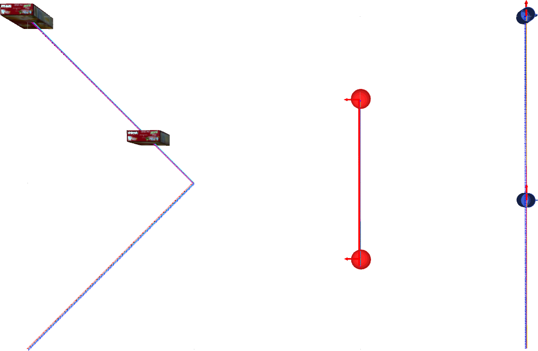
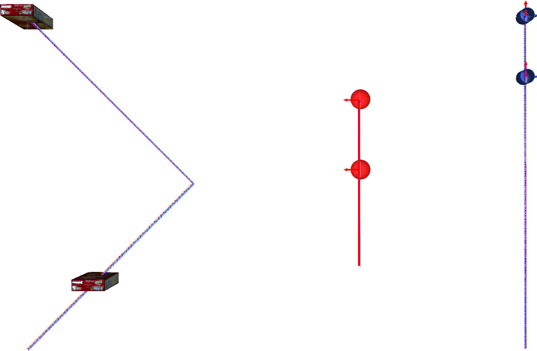
Figure 3: Two test sets randomly picked from the trajectories (lower objects; one valid and one invalid)
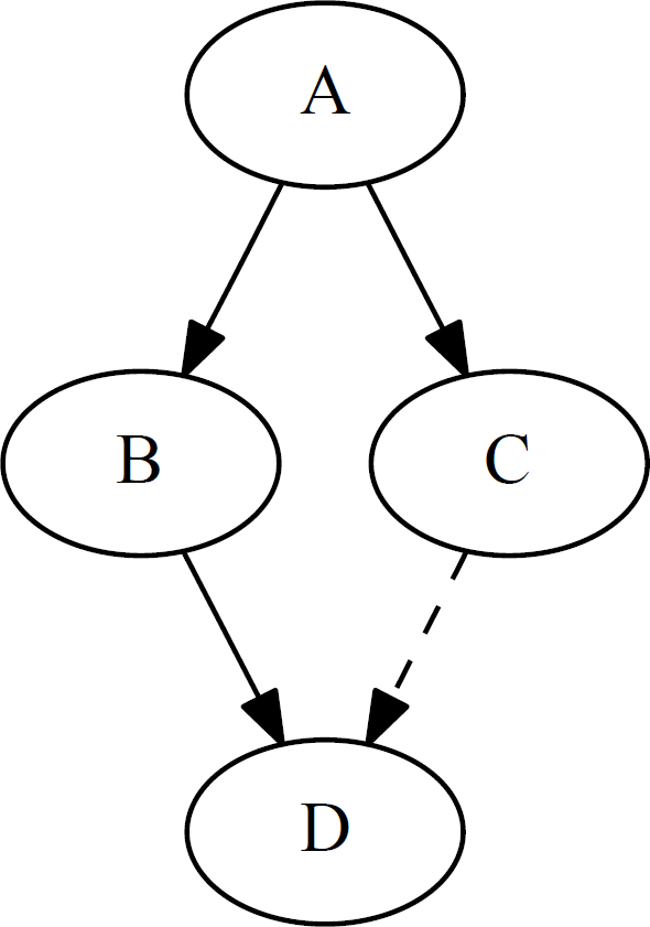
Figure 4: There are relations between B and D as well as C and D. B and C are called the parents of D. Each node can have several parents in graphs generated by combinatorial optimization, other than in the trees from the heuristical method.
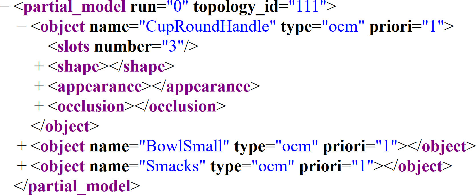
Figure 5: A partial model. Compare to the complete model above. Only the OCM part is used here.
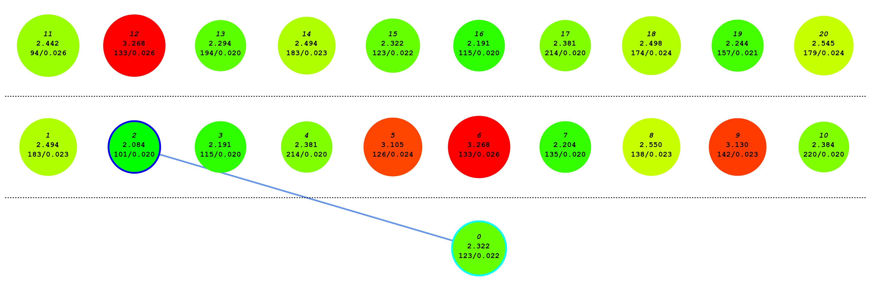
Figure 6: A short optimization history, visualized through circles representing relation sets. The size depends on their cost (middle value), their colour on their average recogntion runtime in s (lower right value). The value in the lower left is the number of recogntion errors. Dotted lines divide optimization steps. A bright blue circle indicates the set selected in each step, a dark blue one the final, optimal set. The blue line shows the path taken through the sets.
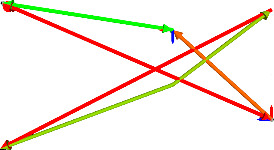
Figure 7: Intermediate visualization of the recognition results of a triangle shaped set against two test sets.
